Introduction#

For this project, we have been given a dataset that will be used to train a model for intrusion detection on networks. I will go through the following steps:

1. Data Preprocessing: • Analyze the dataset to understand the distribution of classes. • Handle missing values, if any. • Encode categorical features appropriately.
2. Feature Selection: • Perform feature selection or dimensionality reduction to improve model performance.
3. Model Selection: • Experiment with at least one different machine learning algorithms (e.g., Decision Trees, Support Vector Machines, Neural Networks). • Justify your choice of algorithms based on theoretical knowledge and the characteristics of the dataset.
4. Model Evaluation: • Evaluate the performance of your models using metrics such as accuracy, precision, recall, F1-score, and confusion matrix. • (in Bonus) Compare the performance of different models and provide a comprehensive analysis.
5. Hyperparameter Tuning: • Use techniques like Grid Search or Random Search to optimize the hyperparameters of your chosen models.
6. Report: • Document your approach, decisions, and results in a detailed report. • Include visualizations of your findings, such as feature importance, performance metrics, and decision boundaries.

For this project, my random seed is 21.

Link to the Jupyter Notebook: https://github.com/Sharper8/Intrusion-detection-with-Machine-Learning.git

Report#

Data preprocessing#

Our original data has 43 dimensions, 10 gets dropped with the random selection. We are going to work with the following data:

• Number of rows: 50604
• Number of columns: 33
• Column names: [‘duration’, ‘protocol_type’, ‘service’, ‘flag’, ‘dst_bytes’, ’land’, ‘wrong_fragment’, ’logged_in’, ’num_compromised’, ‘root_shell’, ‘su_attempted’, ’num_file_creations’, ’num_shells’, ’num_access_files’, ’num_outbound_cmds’, ‘is_host_login’, ‘is_guest_login’, ‘count’, ‘srv_count’, ‘serror_rate’, ‘srv_serror_rate’, ‘rerror_rate’, ‘srv_rerror_rate’, ‘same_srv_rate’, ‘diff_srv_rate’, ‘srv_diff_host_rate’, ‘dst_host_count’, ‘dst_host_srv_count’, ‘dst_host_same_srv_rate’, ‘dst_host_serror_rate’, ‘dst_host_rerror_rate’, ‘dst_host_srv_rerror_rate’, ‘outcome’].

The goal is to train a machine learning model that correctly maps the packets into the different classes of OUTCOME which represents the packet type between the following 20 classes:

• All labels in dataset: [‘back’ ‘buffer_overflow’ ‘ftp_write’ ‘guess_passwd’ ‘imap’ ‘ipsweep’ ’land’ ’loadmodule’ ‘multihop’ ’neptune’ ’nmap’ ’normal’ ‘pod’ ‘portsweep’ ‘rootkit’ ‘satan’ ‘smurf’ ’teardrop’ ‘warezclient’ ‘warezmaster’]

Let us begin by doing a report on the data, to get familiar with the material we have.

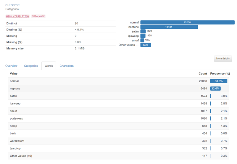
There is 50 000 lines of data, and 33 columns, 2 classes represent 85% of the data: “normal” or “neptune” traffic :

Feature Selection#

Our final goal is to train the model to be able to differentiate between normal traffic and anormal traffic, and we can try to go further by letting the model classify which type of attack it is the most probable to be. In our case, normal traffic might be overrepresented if we wanted to differentiate normal/anormal traffic. However, since we want the model to classify packets into 20 classes, there is a risk that the less represented classes in the training will never be detected (13 classes are below 1%). he profiling report shows a constant “num_outbound_cmds” that we can drop for more efficiency during training.

I choose not to drop duplicate rows for now, and not to drop any more columns, as they are potentially still representative data of a real scenario.

For features especially, even if one feature is highly imbalanced, it could have an impact on classification, for example if 1% of data has a trait, but all of those 1% reveals themselves to be all from the same class, that could indicate that this rare data is really informative. (We will see in the last part however that some features don’t seem to be really useful and could be dropped, but I couldn’t identify it right away and I didn’t wanted to drop important features only based on their imbalanced character)

Model Selection#

The Goal is to have a model that can classify packets in the 20 classes, and that could be usable in the long run in real use cases for example in either IPS/IDS, forensics, or even for research. We would in that context prefer to have a false positive that a false negative; and be able to detect new attacks that the model was never trained on. In fact, if this model is used for attack mitigation or intrusion detection for example, it would be better to miss-categorize normal traffic with suspect behavior than the opposite, because letting an attack through would be a bigger danger.

Since the number of lines in the data is not too big (~50 000), we are not limited by the computation cost of training depending on the model. First, since our goal is to classify, we have the choice between the following models:

• Decision Trees
• Muti Layer Perceptron
• Logistic Regression
• KNN

I chose to use the Multi-Layer Perceptron due to the following:

• I chose to keep the 20 classes; thus, a decision tree would have to be more complex and have more depth, which is not the most efficient in my opinion
• KNN might be less appropriate because of the high dimensionality, since I chose to let the 30 features it might perform worse or could require more hyperparameter tuning
• The problem of classification based on packets may not be linear, thus an LR model may not catch that relation effectively, and we would prefer to have a bit more complexity for better performance
• Multi-Layer Perceptron is better fitted than the previous choices because I have a lot of features with a lot of classes, which are most probably not discriminable linearly. Multi-Layer Perceptron should be better for finding a generalization or a general pattern for each class, if our goal is to have a broad detection method that is reusable, then we should choose the model the less prone to overfitting but better for generalization and complex (nonlinear) classification.

The model training and prediction will be implemented with the following lines of code:

——— Model: Multilayer Perception model ———#

from sklearn.neural_network import MLPClassifier from sklearn.datasets import make_classification

train the model and make predictions#

mlp = MLPClassifier(hidden_layer_sizes=(100,), max_iter=300, activation=‘relu’, solver=‘adam’, random_state=random_seed) mlp.fit(X_train, y_train) y_pred_mlp = mlp.predict(X_test)

We will then use decision tree to help us visualize what features or characters are determinant, and then do a second round of hyperparameter selection if necessary; then propose in bonus the results for other models.

Model Evaluation#

After the training and tests are done, we can evaluate the performance of the model with the following lines of code:

Which gives the output:

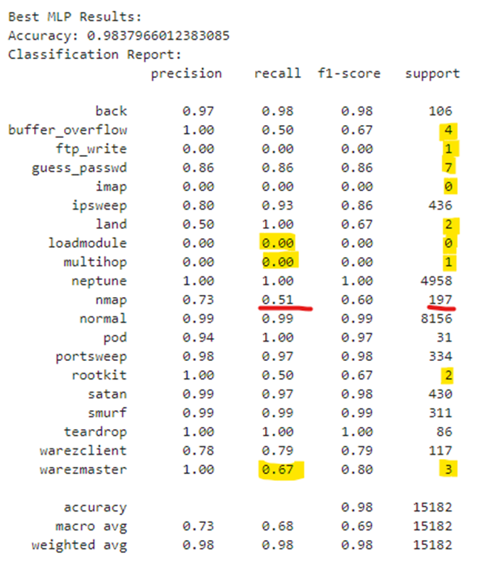
The global accuracy is correct with 98% precision. But in our case, since the false negatives are more important than false positives, we should aim to maximize recall as well.

However, recall could be higher especially on the class n°10 nmap that has 200 occurrences. This could imply either that the training set doesn’t have enough data, and it was all in the test set, or that it is really difficult to differentiate it from others. We can print the confusion matrix to understand better where the errors that were made:
In the actual state, we could still differentiate between normal traffic and the malicious traffic, the 17 other classes. However, some cases are still misclassified as normal traffic, which would be a problem for IDS/IPS automation: n°16-> warezclient, 13->satan, 8-> nmap; are the riskier types of traffic/attack or the most difficult to detect with the model)

These problems could arise from the fact that we don’t have enough data to train the MLP correctly: it could be possible that majority of the data of some classes are in the test set and not in the train set, or that they are separated evenly but there is not enough lines with a specific class. We can try to make the performance better by tuning the MLP hyperparameters, because there is no way to know as if we have chosen the best one on the first try.

Hyperparameter Tuning#

The parameters that we can tweak for the MLP are the learning rate, iteration number, hidden layer neurons, and the activation function. If this is not sufficient and the performance boost is not good enough, we could try to tweak the data:

• By separating evenly, the classes in the train and test set so the MLP can have enough data to train on
• By bringing the low populated classes together into an “other malicious” class, that will serve to mitigate the risk of getting misclassified data in normal traffic if they are malicious. (this method could not work well if the traffic types are different and hard to differentiate, it should be picked better than just with the occurrence, like on what layer they operate, or find a higher class. I don’t have enough knowledge of all the 20 attacks however, so we will still try it and pick the best solution.)

I chose to show all the steps of my reasoning for the parameter’s optimization, the total execution time was 20 minutes on my laptop. I chose to add DEBUG conditions to bypass the grid search and have the code executing in 7 seconds. The initial code for the grid search is still present in the code, as it was a requirement for the code to be 100% replicable.

As a first step, we can add a grid search to try multiple combinations of parameters for the MLP:

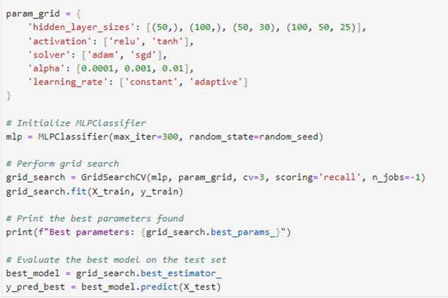
This gives us:

with the following performances:

Here is a comparison between both recall:

Basic MLP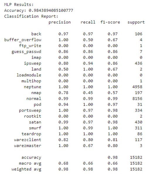 Optimized MLP

In real case, I would stop there: the grid search is computing-intensive and takes 10 minutes on my laptop. However, let’s try to understand what impact a different feature selection/preprocessing could have on the results.

Since the performance of the model wasn’t improved significantly, we can try to review the data selection and pre-processing: both feature selection and redundancies could be cleaned to try balancing all the classes in the data.

However, I can’t be sure about what features and lines I should remove or not, so I can try to visualize what features are the most important for the decision, with for example a decision tree.

First, let’s train a decision tree to see the importance of each feature:
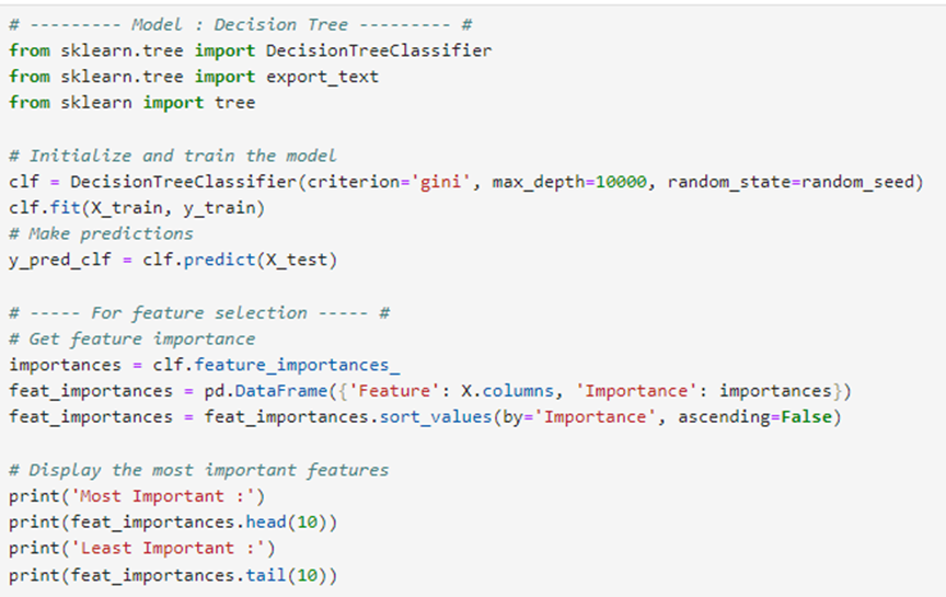This code gives us the data that is not useful for classification with a decision tree model. 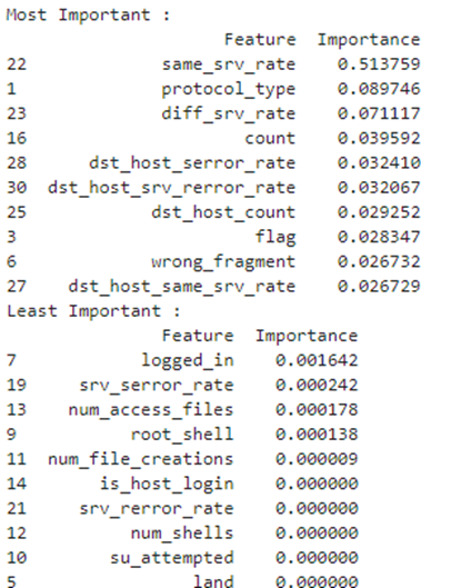While MLP and the decision tree are two totally different models, the importance factor of the tree can help us understand and validate what we might want to drop. When we cross check with the data report, we can see that all of these features are really imbalanced (all over 85%) which can justify to try dropping them and experiment with the results of mp training on this new dataset:
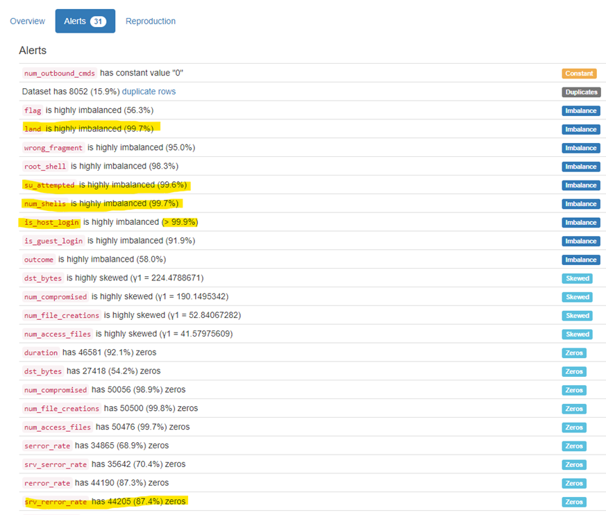We then drop all the features with the importance of 0 and we can re-try the grid search :

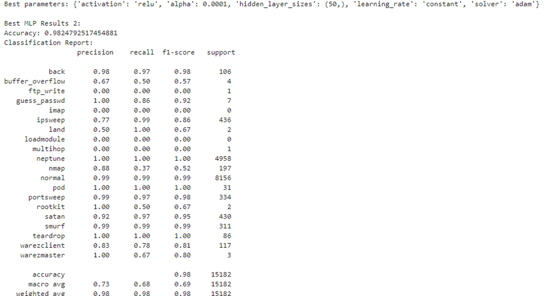
We can see that the accuracy is slightly worse, but the recall is better, by detecting a ‘rootkit’ (the data on rootkit might not be enough populated, this is why it has a limited impact on the weighted avg): 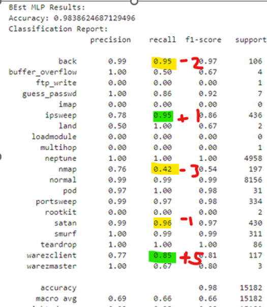Old grid search n°1 New Grid Search n°2

Thus, we need to stratify the data as well which means that we separate evenly the data across both test and training sets, to limit the data shortage in the training set for the MLP:

Perform the train-test split with stratification#

X_train_3, X_test_3, y_train_3, y_test_3 = train_test_split(X_3, y_3, test_size=0.3, stratify=y_3, random_state=random_seed)

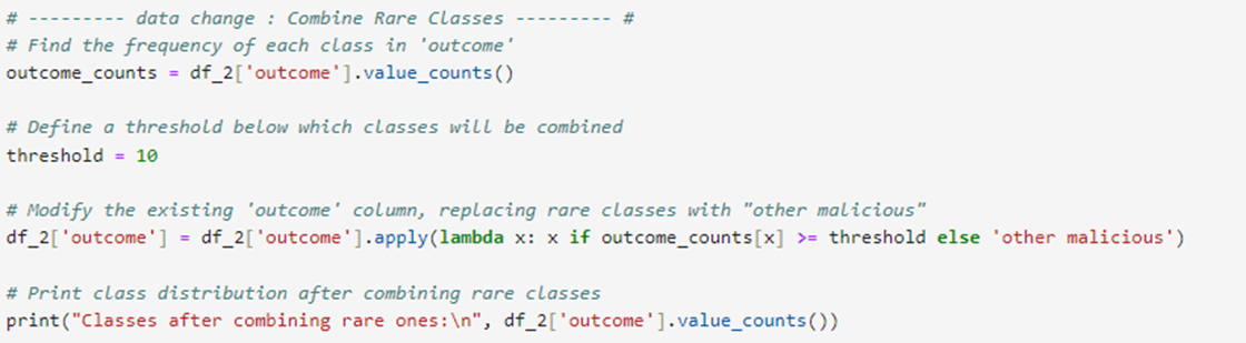
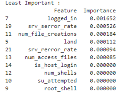
We will put every attack with not enough data (we arbitrary chose 10 population here) and put them in a new class “other malicious”. This could improve the performance for distinguishing normal/anormal traffic but at the cost of losing specificity and information (we lose 8 classes each with their specificity). 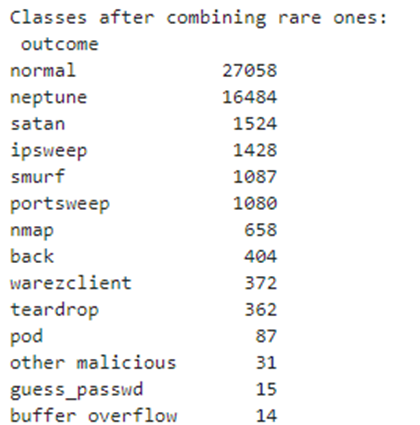We then re-train a tree with those classes to drop the “unimportant” features (note that srv_rerror_rate is not 0 anymore, which could indicate a mistake on the previous step): and re-launch a grid search with this new data frame. The best parameters are the same as other grid search:

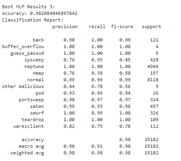
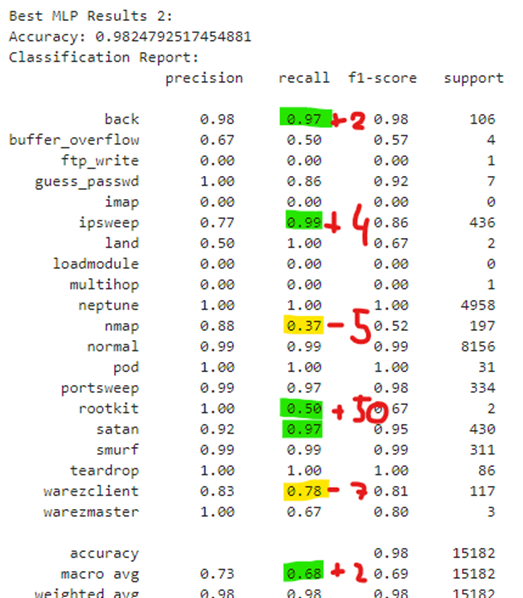
By doing so, we have improved the recall rate for the entire MLP without sacrificing the precision too much. Here is a comparison with the first iteration:

Old grid search n°1 New Grid Search n°3

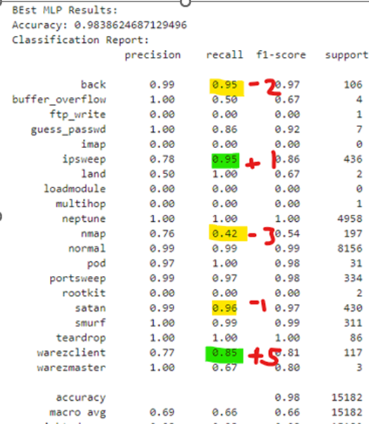
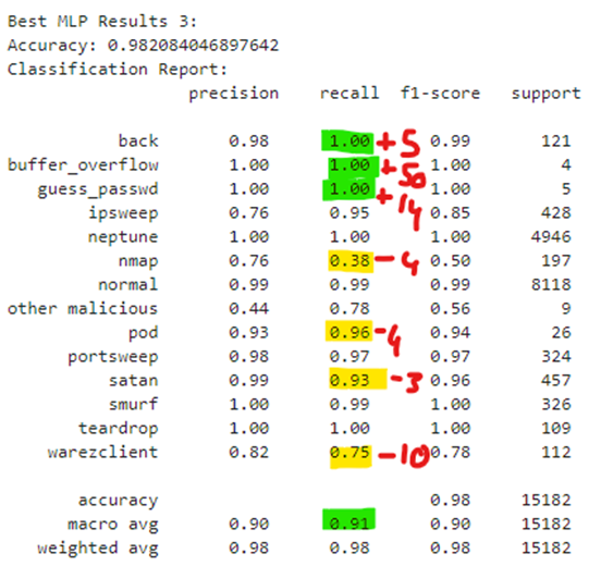
This doesn’t mean however that this last MLP is fundamentally better than the previous ones, because the data is different: we have only sorted the data shortage for rare classes and stratified it. If we take a closer look, it seems this data frame made every low populated class better detected, at the expense of higher populated classes. This is not sure if it would be more viable for IDS/IPS.

Conclusion#

In conclusion, we understood all the steps to build a Multi-Layer Perceptron classifier that could be used for intrusion detection. We have detailed every step of the process, from data pre-processing to model selection, evaluation and multiple iteration for optimization of its performance.

In my opinion, the performance of all the models is impressive, considering the scarcity of population on certain classes and the relative simplicity of the data frame.

In a real use case, I think I would keep the highest scoring model, with the data selection stratified and with the best recall possible to avoid false negative. This project has been interesting and reminds us that even if artificial intelligence is a polyvalent way of automating tasks, we still can’t totally rely on it for risky subjects.

Bonus#

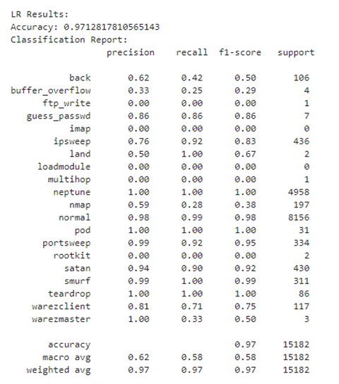
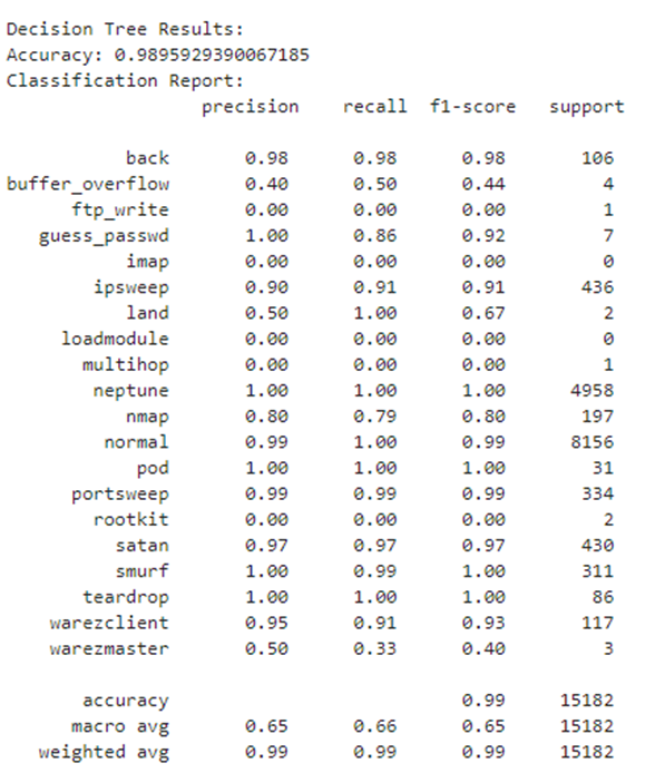
Here are the performances of the other models for comparison purposes (Note that those have not been hyperparameters tuned to get the maximum precision and recall.):

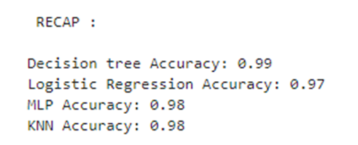
• Logistic Regression: Same accuracy, worse recall, this was expected as explained before.
• Decision Tree: better accuracy and equivalent recall. Wisest choice or overfitting?
• KNN: Same accuracy and slightly worse recall could be interesting with dataframe n°3.
  

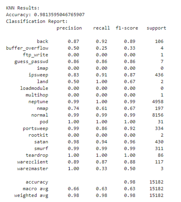
Recap of all model’s performance and comparison: